Build an End-to-End Encrypted Shazam Application Using Concrete ML

Shazam's algorithm, detailed in a 2003 paper, involves users sending queries to its servers for matching in its central database—a prime scenario for applying FHE to protect user data. We challenged bounty participants to create a Shazam-esque app using FHE, allowing for any machine learning technique or the method outlined in Shazam's original paper.

The winning solution structured its work into two steps:

• Song signature extraction on cleartext songs, performed on the client side
• Look-up of the encrypted signatures in the music database on the server side

The solution is based on a custom implementation using machine learning models, and matches a song against a 1000-song database in less than half a second, while providing a client/server application based on the Concrete ML classifiers.

‍

First step: extract the audio features.

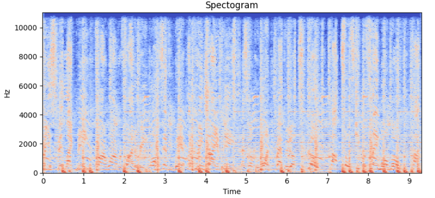
Spectrograms are a popular approach to extracting features from raw audio. Spectrograms are created by applying the Fourier transform to overlapping segments of an audio track. They are resilient to noise and audio compression artifacts, common in recordings made by phones in noisy environments. Furthermore, by normalizing the amplitude spectrum it is possible to add invariance to audio volume.

‍

Second step: convert the original Shazam algorithm to FHE.

The original Shazam algorithm utilizes spectrograms, identifying local maxima within these and recording their time and frequency of occurrence.

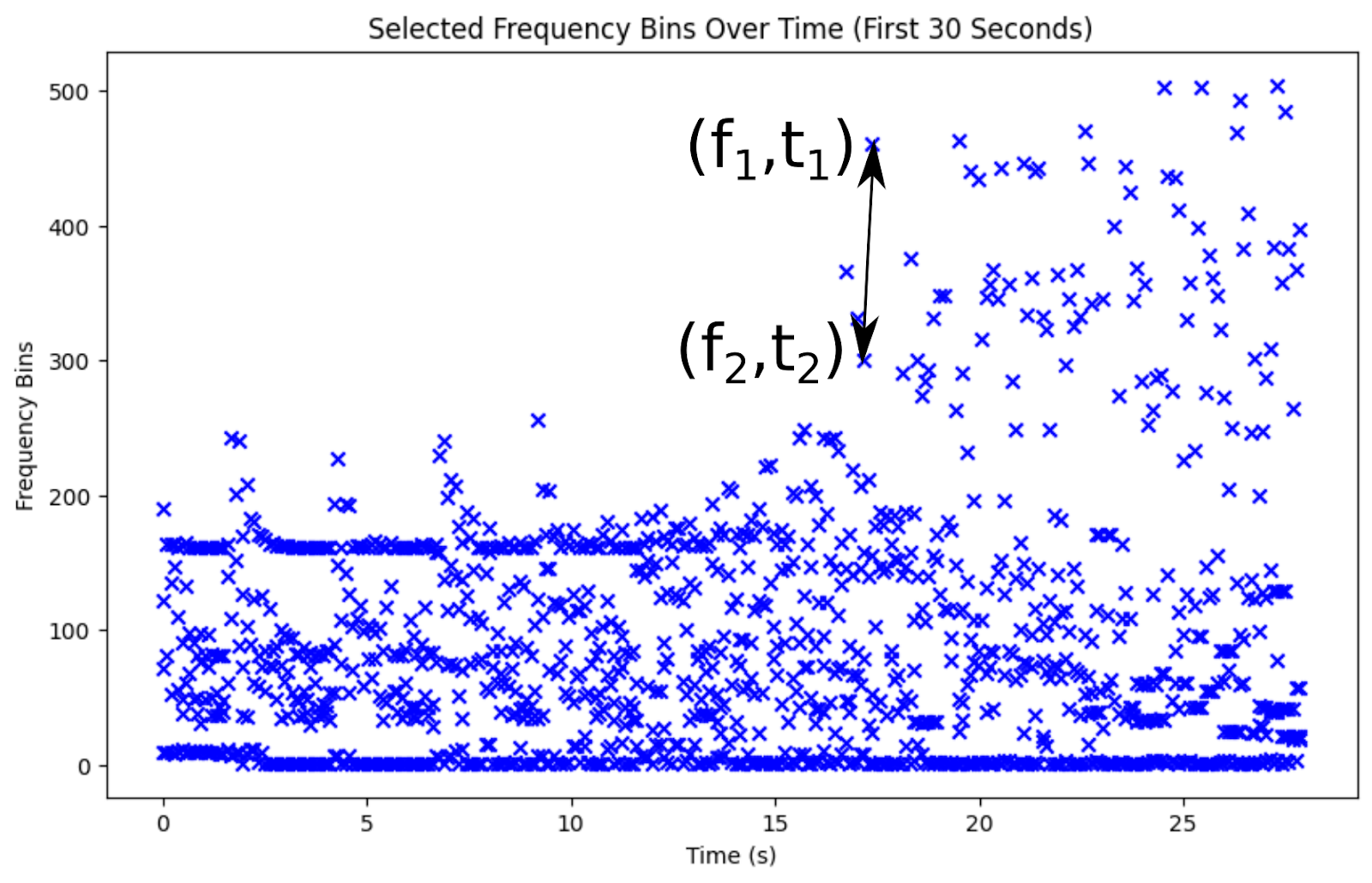
Peaks in the spectrogram are key, yet identifying individual songs from billions demands even greater specificity. The Shazam paper highlights the use of peak pairs, close in time, to distinguish songs from brief recordings. A collection of such peak pairs, marking high-amplitude peaks with their frequencies and the time gap between them, uniquely identifies a song. Encoding frequencies on 10 bits and the time delta on 12 bits results in a 32-bit number which can be considered as a hash of the song.

Tutorial

In the winning solution, the author cut up the song in half-second windows, generated spectrograms for each, and extracted Mel-frequency cepstral coefficients (MFCC) from these. The coefficients extracted from 15-second segments of a song are compiled in a single song descriptor.

For each song in the Shazam database, a few dozen feature vectors are extracted and assigned the song's ID as their label. Following this, a multi-class logistic regression model is trained using Concrete ML, designed to classify each feature vector and match it to its corresponding song ID.

It's worth noting that the linear models in Concrete ML operate without the need for programmable bootstrapping, making them significantly faster than methods that require bootstrapping.

With this design, the model compared a query song against the entire database in less than half a second, and obtained a 97% accuracy rate. Let's take a look, step by step, to iamayushanand's solution.

Feature extraction

Feature extraction is done in two steps:

• Computation of MFCC using librosa
• Aggregation of features by song

Compute features function.

This function returns a matrix of features. The i-th entry in [.c-inline-code]feats[.c-inline-code] is the sum of MFCC coefficients in a 500ms window, as the entire song is divided into 500ms chunks.

import numpy as np
import librosa
def compute_features(y):
    feats = []
    win_sz = SAMPLE_RATE//MFCC_SAMPLES_PER_SEC
    for i in range(len(y)//win_sz):
        y_chunk = y[win_sz*i:win_sz*(i+1)]
        mfcc_f = np.sum(librosa.feature.mfcc(y=y_chunk, sr=SAMPLE_RATE), axis=1)
        feats.append(mfcc_f)
    return feats

‍

Add features function.

This function retrieves features for a specified song and appends them to a [.c-inline-code]feature_db[.c-inline-code] array along with its [.c-inline-code]id[.c-inline-code].

feature_db = []
def add_features(y, id):
    feats = compute_features(y)
    for feat in feats:
        feature_db.append((feat, id))

Load 3 minute samples from each song from the specified directory and build the feature database.

idx = []

for dirpath, dnames, fnames in os.walk(MUSIC_DB_PATH):
    if len(idx) >= NUM_SONGS:
        break
    for f in fnames:
        try:
            song_name = f
            song_path = os.path.join(dirpath, f)
            y, sr = librosa.load(song_path, sr = SAMPLE_RATE, duration = 180)
            if song_name not in idx:
                idx.append(song_name)
                print(f"id: {idx.index(song_name)}, song_name: {song_name}")
            add_features(y, idx.index(song_name))
            if len(idx) >= NUM_SONGS:
                break
        except:
            pass
print(f"Total number of features to train on: {len(feature_db)}")

_{id: 0, song_name: 135054.mp3}

_{id: 1, song_name: 135336.mp3}

_(...)

_{id: 398, song_name: 024364.mp3}

_{id: 399, song_name: 024370.mp3}

_{Total number of features to train on: 23770}

After feature extraction, each song is represented by an ensemble of 60 feature vectors.

Evaluation function

The evaluation function computes the accuracy, hence, the percentage of queries that return the correct song. Thanks to the [.c-inline-code]predict_in_fhe[.c-inline-code] parameter, the evaluation can either execute on encrypted data or on cleartext using FHE simulation.

def evaluate(model, model_config, truth_label, samples_path, predict_in_fhe = False):
    evaluation = {**model_config}
    evaluation["Inference Time"] = 0
    evaluation["Accuracy"] = 0

    if predict_in_fhe:
        evaluation["Inference Time (FHE)"] = 0
        evaluation["Accuracy (FHE)"] = 0

    for dirpath, dnames, fnames in os.walk(samples_path):
        for f in fnames:
            if f not in truth_label:
                continue
            
            print(f"processing {f}")
            song_path = os.path.join(dirpath, f)
            y, sr = librosa.load(song_path, sr = SAMPLE_RATE, duration = 15)
            features = compute_features(y)

            start = time.time()
            preds = model.predict(features)
            end = time.time()

            evaluation["Inference Time"] += end-start

            class_prediction = np.argmax(np.bincount(preds))
            if np.bincount(preds)[class_prediction] < 5:
                class_prediction = -1 # Unknown Class
            
            
            
            evaluation["Accuracy"] += (class_prediction == truth_label[f])
    
            if predict_in_fhe:
                start = time.time()
                preds = model.predict(features, fhe="execute")
                end = time.time()

                evaluation["Inference Time (FHE)"] += end-start

                class_prediction = np.argmax(np.bincount(preds))
                if np.bincount(preds)[class_prediction] < 5:
                    class_prediction = -1 
                
                
                
                evaluation["Accuracy (FHE)"] += (class_prediction == truth_label[f])
    evaluation["Accuracy"] /= len(truth_label)
    evaluation["Inference Time"] /= len(truth_label)

    if predict_in_fhe:
        evaluation["Inference Time (FHE)"] /= len(truth_label)
        evaluation["Accuracy (FHE)"] /= len(truth_label)
    return evaluation

Models

The winning solution is based on Logistic Regression which is fast and easy to use. During development several models were tested to evaluate the speed/accuracy tradeoff before finally settling for Logistic Regression.

from concrete.ml.sklearn import LogisticRegression as ConcreteLR
from sklearn.model_selection import train_test_split
concrete_configs = [ {'n_bits': 8}]
concrete_models = [ConcreteLR(**concrete_configs[0]) ]
for model in concrete_models:
    model.fit(features, ids)
    model.compile(features)

First we evaluate the models on a small hand-curated recording sample set. This was created by playing the music on a phone and recording it through a laptop microphone.

#truth_label = {"sample1.mp3": idx.index("Alena Smirnova - Lyric song.mp3"),
#               "sample2.mp3": idx.index("Edoy - Topaz.mp3"),
#               "sample3_recorded.m4a": idx.index("Pierce Murphy - Devil In A Falling Sky.mp3")}
truth_label = {
               "133916.mp3": idx.index("133916.mp3"),
               "135054.mp3": idx.index("135054.mp3"),
               "024366.mp3": idx.index("024366.mp3"),
              }

print(truth_label)
evaluations = {}
model_names = [ "ConcreteLR"]
for i, model in enumerate(concrete_models):
    evaluations[model_names[i]] = evaluate(model, concrete_configs[i], truth_label, TEST_SAMPLE_PATH, predict_in_fhe=True)

_{processing 135054.mp3}

_{processing 024366.mp3}

_{processing 133916.mp3}

The evaluation results are compiled in a pandas dataframe that we can print easily. It contains the accuracy and inference latency both on encrypted data and on cleartext data.

import pandas as pd
df = pd.DataFrame(evaluations)
df

Finally, the system is evaluated on the entire dataset.

truth_label_train = {}

for i, id in enumerate(idx):
    truth_label_train[id] = i
evaluations = {}
model_names = [ "ConcreteLR"]
for i, model in enumerate(concrete_models):
    evaluations[model_names[i]] = evaluate(model, concrete_configs[i], truth_label_train, MUSIC_DB_PATH, predict_in_fhe=True)

_{processing 135054.mp3}

_{processing 135336.mp3}

_(...)

_{processing 024364.mp3}

_{processing 024370.mp3}

‍

The result on the entire dataset are compelling: the song is correctly recognized 97% of the time, and accuracy on encrypted data is the same as on cleartext data. Furthermore, to recognize a single song out of 1,000 takes only 300 milliseconds.

Comparison with scikit-learn LR model

The winning solution compared the results with the FHE model on encrypted data with respect to a baseline without encryption, implemented with scikit-learn.

from sklearn.linear_model import LogisticRegression

sklearn_lr = LogisticRegression().fit(features, ids)
evaluations["sklearn_lr"] = evaluate(sklearn_lr, {}, truth_label_train, MUSIC_DB_PATH, predict_in_fhe=False)

This experiment shows that the result using scikit-learn is the same as the one using Concrete ML.

Conclusion

We are very thrilled by the innovative approach this solution is using to tackle the challenge of creating an encrypted version of Shazam using FHE. Once again, the developers who took part in this bounty challenge have shown us that FHE can be the cornerstone for privacy protection, and that it has the power to enhance privacy in the popular apps used by millions. Check out all other winning solutions and currently open bounties on the official bounty program and grant program Github repository (Don't forget to star it ⭐️).

Additional links

• Our community channels, for support and more.
• Zama on Twitter.